Search for an answer or browse help topics

The Back Testing screen can be loaded from the Alerts menu in the Main Menu.
Back Testing is a method that traders use to test their trading strategies against historical market conditions. Knowing how much profit or loss a trading system generated in the past may help prevent or reduce the risk of loss in real trading.
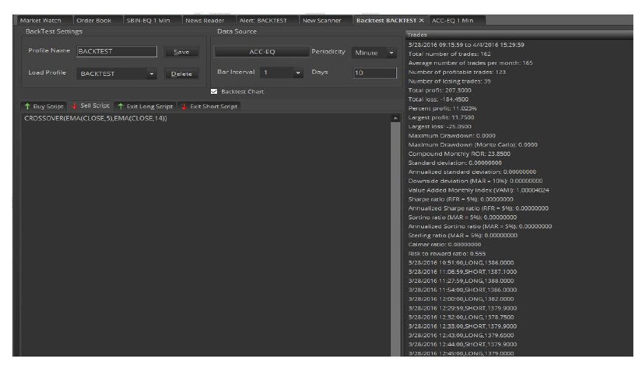
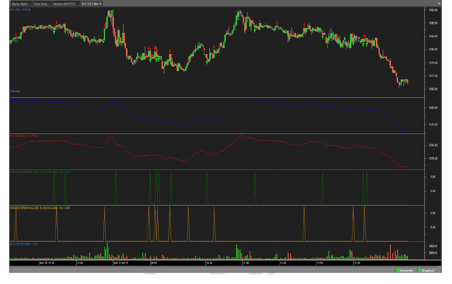
The Abacus Back Testing engine can calculate a user’s trading system's performance using nearly two-dozen scientific profit, loss, and risk measurements. Abacus allows users to specify individual instructions for buying, selling, holding, and exiting his/her simulated trades. To run a Back Test, simply enter and verify user buy, sell, and exit scripts then click the Back Test button. The Buy Script is a set of instructions for buying (going long) and the "Shell Script" is a set of instructions for selling (going short).
The scripts required on this screen are based on the Abacus programming language. Please refer to the Abacus programming guide for complete details. Click on script guide will open the Tradescript Help document for users to learn how to write Buy, Sell, and Exit scripts.
Users can add symbols by clicking on the Select Symbol button which will open the Select symbol window to select symbols from any of the exchanges to perform the Backtesting.
Back Test Results Overview
Some trading strategies work well on a wide range of securities but work poorly with some securities. Reasons may include poor market liquidity for a particular stock (low volume), high volatility, and other factors. It is a good idea to test the user’s own strategy across a wide range of securities. Just because it isn’t very profitable on one security doesn’t mean it won’t work well with another security.
The values on the backtesting page represent a range of measurements based on the profitability and risk of the user’s trading system when tested with the symbol that user-supplied at the top of the backtest screen. The output on the backtesting results list provides an overall picture of how the user’s strategy might perform if used as a live trading system.
Overview of Back Test Outputs
Total Number of Trades
A total number of trades including buying, sell, and exit trades.
Average Number of Trades per Month
An average number of trades per month, including buy-sell, and exit trades.
Number of Profitable Trades
A total number of profitable trades since the beginning of the backtest.
Number of Losing Trades
A total number of non-profitable trades since the beginning of the backtest.
Total Profit
Total profit since the beginning of the backtest.
Total Loss
Total loss since the beginning of the backtest.
Percent Profit
Percentage of profitable trades since the beginning of the backtest.
Largest Profit
Largest single trade profit.
Largest Loss
Largest single trade loss.
Maximum Drawdown
The maximum account drawdown, defined as the percent retrenchment from equity peak to equity valley. A drawdown is in effect from the time an equity retrenchment begins until a new equity high is reached.
Maximum Drawdown (Monte Carlo)
Same as maximum drawdown, except the test is repeated 5,000 times, with each test introducing a small random slippage. Preferred over regular drawdown.
Value-Added Monthly Index (VAMI)
Reflects the growth of a hypothetical $1,000 in a given investment over time. The index is equal to $1,000 at inception. Subsequent month-end values are calculated by multiplying the previous month’s VAMI index by 1plus the current monthly rate of return.
Where Vami 0=1000 and
Where R N=Return for period N
Vami N = (1 + R N) X Vami N-1
Compound Monthly ROR
The geometric mean is the monthly average return that assumes the same rate of return every period to arrive at the equivalent compound growth rate reflected in the actual return data.
Standard Deviation
Measure the degree of variation of returns around the mean (average) return. The higher the volatility of the investment returns, the higher the standard deviation will be.
Where R I = Return for period I
Where M R = Mean of return set R
Where N = Number of Periods
M R = (∑ R I) ÷ N
I=1
(∑ (R I - M R) 2 ÷ (N - 1)) ½
Annualized Standard Deviation
Standard Deviation X (12) ½
Downside Deviation (MAR = 10%)
Similar to the standard deviation above except the downside deviation considers only returns that fall below a defined Minimum Acceptable Return (MAR) rather than the arithmetic mean. For example, if the MAR were assumed to be 10%, the downside deviation would measure the variation of each period that falls below 10%. (The loss standard deviation, on the other hand, would take only losing periods, calculate an average return for the losing periods, and then measure the variation between each losing return and the losing return average).
Where R I = Return for period I
Where N = Number of Periods
Where R MAR = Period Minimum Acceptable Return
Where L I = R I - R MAR (IF R I - R MAR < 0) or 0 ( IF R I - R MAR ³ 0 )
((S (L I) 2) ¸ N) ½
I = 1
Downside Deviation = ((S (L I) 2) ¸ N) ½
Where NL = Number of Periods where R I - M < 0
Sharpe Ratio
A measure developed by William Sharpe that is defined as the incremental average return of an investment over the risk-free rate. Risk (denominator) is defined as the standard deviation of the investment returns.
Where R I = Return for period I
Where M R = Mean of return set R
Where N = Number of Periods
Where SD = Period Standard Deviation
Where R RF = Period Risk Free Return
M R = (∑ R I) ÷ N
I = 1
SD = (∑(R I - M R) 2 ÷ (N - 1)) ½
I=1
Sharpe Ratio= (M R - R RF) ÷ SD
Sortino Ratio (MAR = 5%)
A return/risk ratio developed by Frank Sortino. Return (numerator) is defined as the incremental compound average period return over a Minimum Acceptable Return (MAR). Risk (denominator) is defined as the downside Deviation below a Minimum Acceptable Return (MAR).
Where R I = Return for period I
Where N = Number of Periods
Where R MAR = Period Minimum Acceptable Return
Where DD MAR = Downside Deviation
Where L I = R I - R MAR (IF R I - R MAR < 0) or 0 (IF R I - R MAR ≥ 0)
DD MAR = ((∑( L I ) 2 ) ÷ N ) ½
I=1
Sortino Ratio = (Compound Period Return - R MAR) ÷ DD MAR
Annualized Sortino ratio (MAR = 5%)
Annualized Sortino = Monthly Sortino X (12) ½
Calmar Ratio
Return/risk ratio. Return (numerator) is defined as the Compound Annualized Rate of Return over the last 3 years. Risk (denominator) is defined as the Maximum Drawdown over the last 3 years. If three years of data are not available, the available data is used.
Sterling Ratio (MAR = 5%)
Return/risk ratio. Return (numerator) is defined as the Compound Annualized Rate of Return over the last 3 years. Risk (denominator) is defined as the Average Yearly Maximum Drawdown over the last 3 years less an arbitrary 10%. To calculate this average yearly drawdown, the latest 3 years (36 months) is divided into 3 separate 12-month periods and the maximum drawdown is calculated for each. These 3 drawdowns are averaged to produce the Average Yearly Maximum Drawdown for the 3-year period.
Where D1 Calmar Ratio = Average Annual ROR /Worst drawdown = Maximum Drawdown for first 12 months
Where D2 = Maximum Drawdown for next 12 months
Where D3 = Maximum Drawdown for latest 12 months
Average Drawdown = (D1 + D2 + D3) / 3
Sterling Ratio = Compound Annualized ROR /ABS ((Average Drawdown -10%))

Simply fill the details, connect your bank account & upload your documents.
Open An AccountYou will be redirected in a few seconds.